Analyzing AWS Costs with SQL
One of the things nobody loves about AWS is billing. Mainly because the more your application is cloud-native, the more unpredictable your bill will become. All that autoscaling and serverless saves you a lot of money, but if there is a massive spike in your app usage, there will also be a spike in your AWS bill. That’s usually a good thing because if you’ve done it right, the opposite is also true, and low traffic means lower costs.
Either way, the more you use AWS, the less useful the default monthly bill becomes. Maybe you have several environments (production, staging, dev, …), or perhaps you have multiple applications. The aggregated view simply becomes a problem, and you start to wonder how much each of those applications costs separately. Then you discover AWS cost allocation tags and cost explorer that can group by service or tags, which also lasts a while before you become unhappy again.
The problem is always the same - the data is not granular enough. Can we somehow get more granular data?
AWS Cost and Usage Reports
CUR is the holy grail of AWS billing. It works by dumping a bunch of CSV files into an S3 bucket, which you can then process however you like. And if you dive into the data dictionary of that report, you’ll realize there is a lot of value to be extracted.
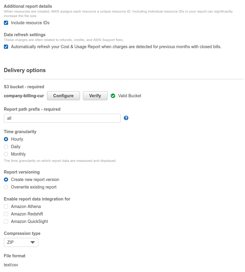
Go to Billing Dashboard > Cost & Usage Reports > Create report
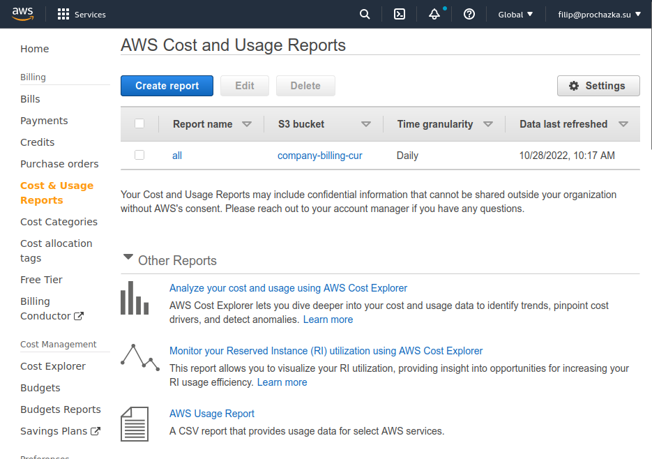
where you’ll configure your report.
And now we wait. Here is where you become sad that you haven’t done it sooner because it dumps only current or previous month. The documentation mentions you can ask the support to have it backfilled, but either way, you’ll be waiting for days to have something to play with.
If you already have a data engineering team in your company and a standard way to create internal dashboards, you can stop reading here. But for the rest of you, I’ll show you a cool and simple way to utilize the data.
Loading the data into a SQL database
I like to do similar experiments locally, so let’s start with a local database in a docker container that we will populate with the CSV files. First, we must download the data from the S3 bucket to work with them locally.
aws s3 sync s3://company-billing-cur ./company-billing-cur
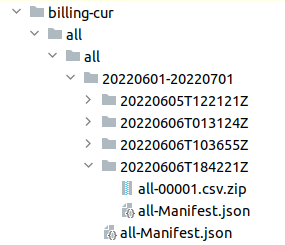
Once you accumulate some data, you’ll notice that AWS keeps dumping the entire billing period over and over, each time with newer data. That’s because it’s giving you partial data for the current month, but also because it can take up to a few days for the billing data to stabilize and become final - you might see updates of the previous month even on 3rd day of the current month. You’ll always want to process the newest dump for each billing period. For the following screenshot, you’d look into the billing-cur/all/all/20220601-20220701/all-Manifest.json because that always contains references to the newest data dump.
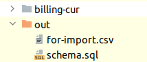
I’ve decided that the quickest way to load the data one time for the initial experiments is to use DataGrip’s “import data from a file” feature, which can natively work with CSVs - I wouldn’t use it for processing a few years’ worths of data, but a month or two should work fine. I also want to have nice column names, so I’ve prepared a python script transform-aws-cur-for-datagrip.py that will find the newest dump per each billing period, transforms the data into the desired shape, dumps schema and lets me do the import manually.
Now that I have something that the DataGrip can nicely import, I’ll spin up a new database instance from docker.
version: "3.4"
services:
  database:
    image: postgres:15-alpine
    volumes:
      - ./.data/db-local:/var/lib/postgresql/data
    environment:
      - POSTGRES_DB=aws-costs
      - POSTGRES_USER=user
      - POSTGRES_PASSWORD=password
    ports:
      - "127.0.0.1:5432:5432"
    command: postgres -c random_page_cost=1.0
Next, I’ll execute the schema.sql to create the table, and then I can start the import. It’s hidden here:
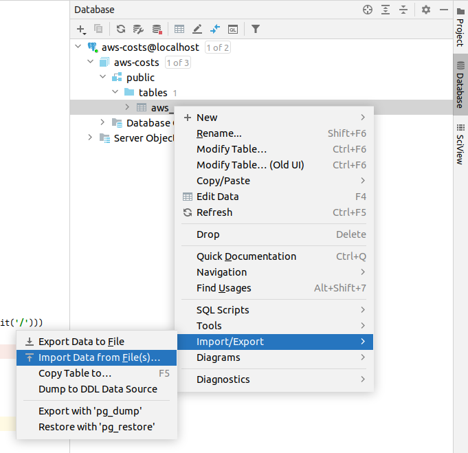
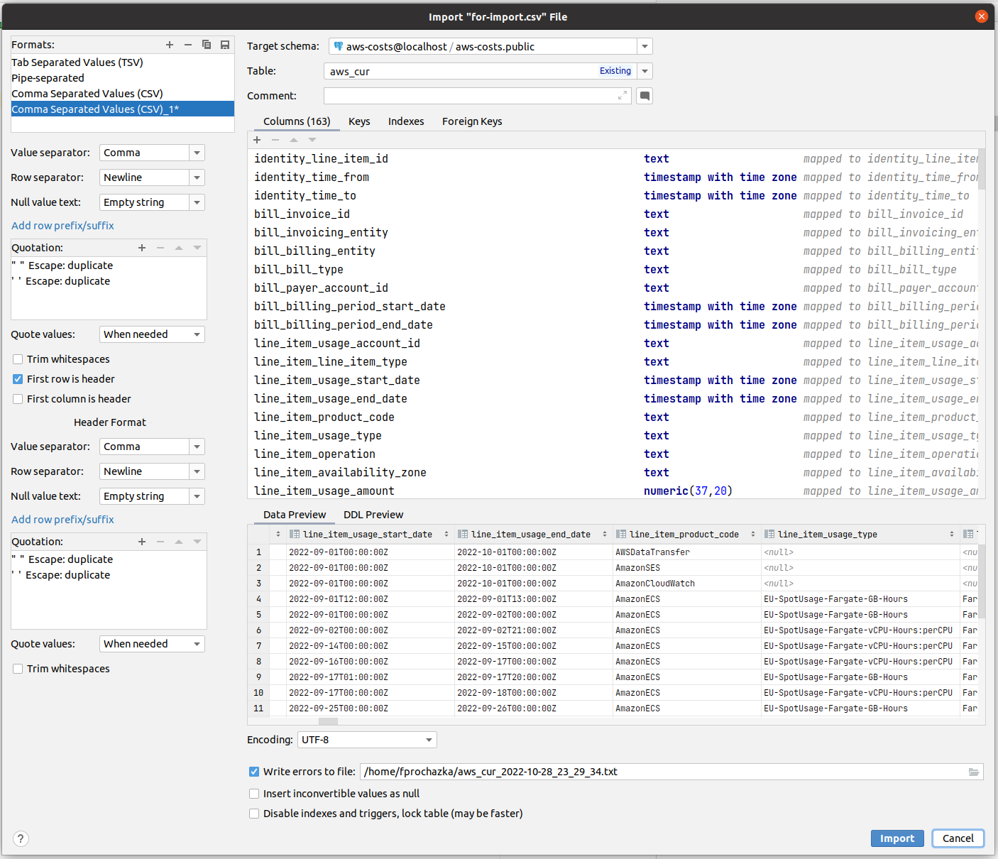
DataGrip might need you to tell it that the first row is CSV headers, but once that’s done, you’ll see that it maps the columns nicely
Then we wait for a bit for the import to finish
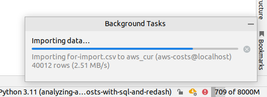
And now you can start poking around in the data!
Access for the rest of the company
I’ll save you the trouble of having to manually compile XLS reports for your boss and tell you right away to skip that step and jump right into to the world of web-based visualization tools. In Cogvio, we’ve used Redash, and in ShipMonk, we’re using Metabase. But operating Redash is IMHO simpler, so I’ll use it to demonstrate this next part. The reason I’m showing these two is that you can keep using them for a long time for free before you outgrow them and need a fully-featured BI analytics platform full of AI and other buzzwords, so let’s return to the real world for now.
Redash has nice guides for deploying it to different places, but for now, let’s stay with docker-compose, and you can figure out how to deploy it to some EC2 on your own. I’ve copied the docker-compose definitions into my project so I’ll have the Redash instance in the same docker network as my “analytical database” with the AWS CUR data.
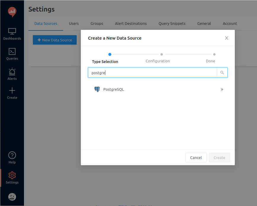
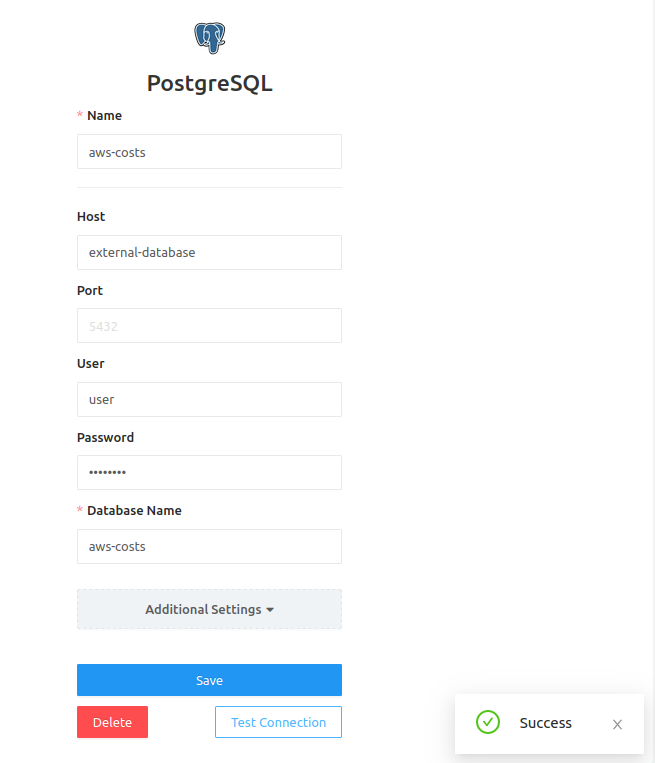
Once you start the instance, you’ll have to create the first admin user. After that, create the data source connection for our analytical database. You can connect Redash to a wide range of data sources and can have multiple connections that you can then query at will and compile into dashboards.
And make sure you test that the connection works.
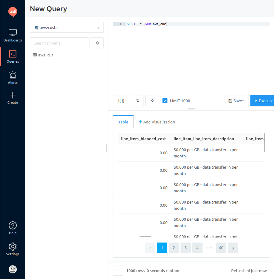
Redash has a pretty solid text editor, but I still like to write queries in DataGrip if I can and only then copy them into Redash for final touches.
CUR dashboards in Redash
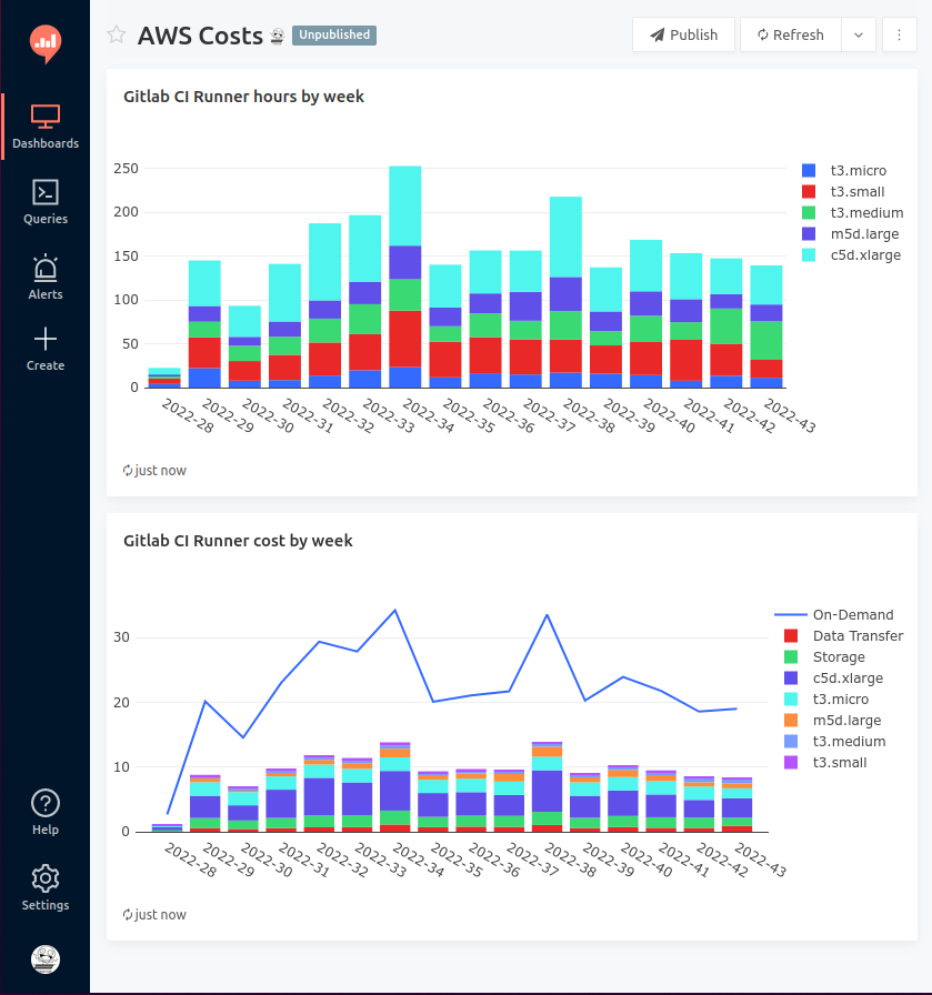
Now that we have Redash prepared, let’s write some queries. Let’s say I want to know how much our Gitlab Runners on the Spot instances cost us every week and how much we’re saving compared to On-Demand prices.
(
    SELECT DATE_PART('year', identity_time_from) || '-' || DATE_PART('week', identity_time_from) as week,
           CASE
            WHEN product_product_family = 'Compute Instance' THEN product_instance_type
            ELSE product_product_family
           END as product,
           SUM(line_item_unblended_cost)::numeric(37, 4) AS cost
    FROM aws_cur
    WHERE resource_tags_user_user_application IN ('Gitlab CI Runner')
    GROUP BY 1, 2
    ORDER BY 1 DESC, 3 DESC, 2
) UNION ALL (
    SELECT DATE_PART('year', identity_time_from) || '-' || DATE_PART('week', identity_time_from) as week,
           'On-Demand' as product,
           SUM(pricing_public_on_demand_cost)::numeric(37, 4) AS cost
    FROM aws_cur
    WHERE resource_tags_user_user_application IN ('Gitlab CI Runner')
    GROUP BY 1, 2
    ORDER BY 1 DESC, 3 DESC, 2
);
And I also want to know how many hours they’re running.
SELECT DATE_PART('year', identity_time_from) || '-' || DATE_PART('week', identity_time_from) as week,
       product_instance_type,
       SUM(line_item_usage_amount)::numeric(37, 4) AS usage_hours
FROM aws_cur
WHERE resource_tags_user_user_application IN ('Gitlab CI Runner')
  AND product_product_family = 'Compute Instance'
  AND product_marketoption != 'OnDemand'
  AND pricing_unit IN ('Hours', 'Hrs')
GROUP BY 1, 2
ORDER BY 1 DESC, 3 DESC, 2;
Create two queries, add a visualization for them, put them in a dashboard, and you’re done!
Once you’re done playing, you’ll obviously want to have all of this deployed somewhere so your colleagues can also see it. But there is still that pesky manual step of loading the CUR data into our analytical database - could we somehow automate that?
Keboola
Once you outgrow hot-glued hacky scripts in AWS Lambdas that keep breaking every other month, you’ll start looking for some solution that can orchestrate data manipulation, transformations and orchestrations for you. I’m not saying Keboola is the best there is, but I’ve seen it in many companies, and it works reasonably well.
With Keboola, we can:
- load the data from the AWS S3 bucket into their platform
- use SQL or Python transformations to clean the data
- write the data into a provisioned Snowflake database
- connect our Redash to that provisioned Snowflake database
- query it the exact same way we did with PostgreSQL, but now with the power of cloud
If you’re cheap, you can use it without Snowflake, but that would be a shame because even though Snowflake is pretty expensive, it’s also extremely fast for analytical queries, which is exactly what we’re doing here.
Also, since the smart people in Keboola know the value of AWS CUR, they’ve prepared a plug-and-play component that correctly extracts the data from your AWS account for you, so you don’t have to code anything, and they’ll be maintaining it for you.
The ideal state
My main point was to show AWS CUR and Redash. You don’t need Keboola if you’re only going to process CUR. Alternatively, AWS can pipe the CUR into Athena or Redshift, which can also be queried from Redash. But suppose you want to tackle data analytics problems seriously. In that case, you will need some data ops platform sooner or later, and I’ve only ever seen Keboola in the companies I’ve worked for, so I don’t have better advice for you right now.
So what should all of this ideally look like if we put it together?
- Setup the AWS Cost and Usage Reports
- Keboola orchestration will regularly load it using their extractor
- The orchestration will write it into a Snowflake database
- Redash is connected to that database and can query it
- Your colleagues can access the Redash dashboards, which show the newest data
And now you have visibility into your AWS bill.
Autor: Filip Procházka